Create frames

Create frames using FRAME()

Typically, you create a frame by using the FRAME() function, which references a cell range with tabular data.

The following is an example of how to create a frame.

1. Create an invoice in the spreadsheet, like the one in the figure below:

   

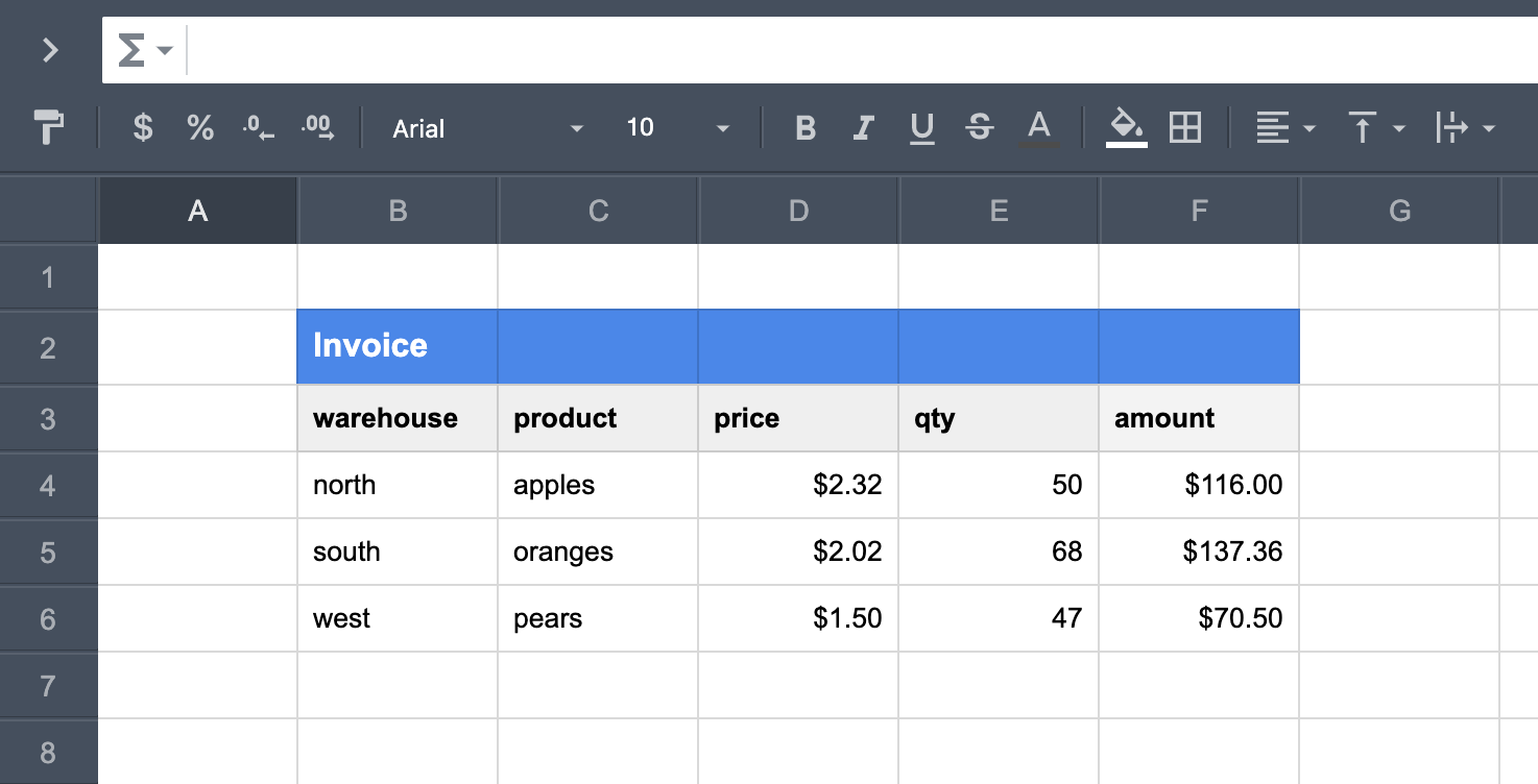
2. In an empty cell, enter a formula with the FRAME() function referencing the range. For example:

   =FRAME(B3:F6)

   

   The cell now contains a frame.

Specify column headers

The second parameter in the Frame function, namesOnFirstRow, defaults to true, which means that the first row of the referenced range is used as column headers in the frame.

If you set the parameter to false, the first row is considered as part of the frame rows, and the column headers in frame have names, like column1, column2, and so on.

Auto-detect the bottom boundary

The third parameter, auto, is used to enable or disable automatic frame update by detecting the bottom boundary. The bottom boundary is determined by an empty cell in the first column range of the referenced range. Default is false. If the auto parameter is set to true, every time a value is added to the first column of the referenced range, the frame is automatically updated.

If you set auto to true, you can reference only the first row in the range: All the rows underneath will be detected automatically according to the values in the first column, and the frame will be updated accordingly.

Create frames using literals

You can create a frame using frame literals:

• Create an empty frame using the following formula

={}

• Create a single-row frame

={"a","b","c"}

• Create a frame with multiple rows.

={"a","b","c"; "d","e","f"}

Try it now